Zoom Notes: Repeating Code
Semester 1, 2022
Associated Material
Module: Module 08 - Iteration
Readings
Topics
Iteration Use Cases
For loops
- Syntax
- Sequence options
- Loop driver variable
- Nested for loops
While loops
- Syntax
- Loop conditions
- Infinite while loops
Alternatives for single function loops
- Map family
- Apply family
Exercises
Loop Driver Practice
Write a for loop that prints the even numbers between 2 and 20. That is, you should print 2, 4, 6, 8… There are multiple ways to achieve this outcome. Get more practice working with loop driver variables by trying to find two different solutions. Hint: If you’ve never used the modulo operator, this is a good time to learn (see for example, https://www.geeksforgeeks.org/r-operators/). Repeat the exercise, with a while loop.
Modeling and simulation with stochasticity
Mathematical modeling is a discipline of study where complex, stochastic phenomena are described using deterministic, empirically testable systems. These systems often involve advanced mathematical techniques. For example, one can define a mathematical model for the response of an architectural design to ground disturbances, and use it to predict the ability of the building to withstand earthquakes of varying intensity. Or one can model the effect of habitat loss on a prey species and use that to predict impacts on an entire food chain.
Because such systems are generally stochastic (i.e. there is random variability in their behaviour), modeled effects are usually simulated many, many times, and a distribution of outcomes produced. While the code required to simulate a system can be very complex, the process of running it many times and accruing the results is easy – just use a for loop.
For example, we have used the function rnorm to randomly
select a single value from a normal distribution. In a mature language
like R, we can assume that this function behaves correctly, but this is
a testable claim. If we were to select many, many single values with
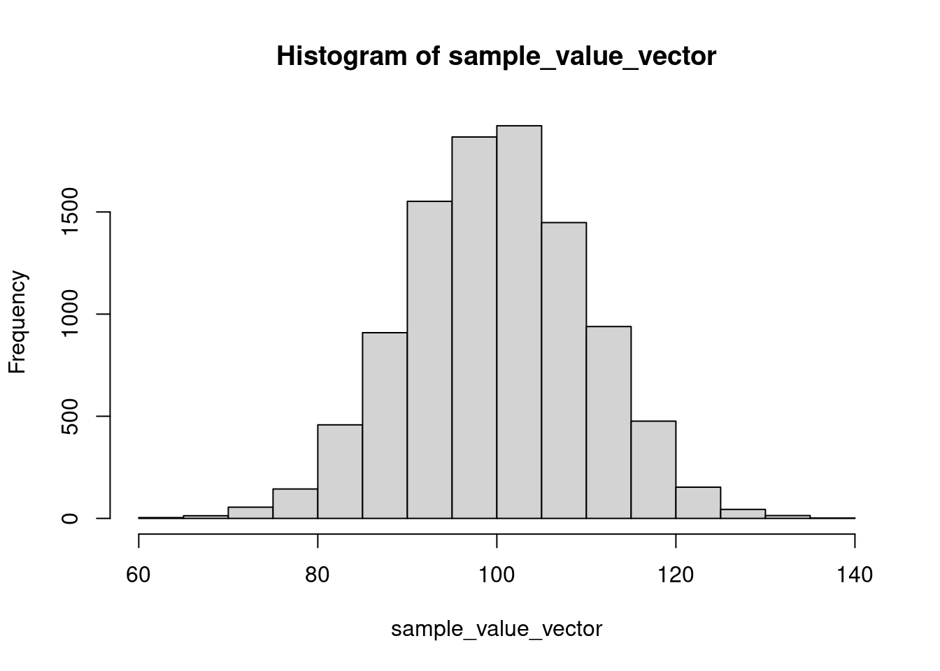
rnorm and plot them, we would expect them to be normally
distributed. (Note that is is actually possible to select multiple
values with rnorm without looping, but we will ignore that small fact
for this example.) This simple simulation illustrates the
loop-compute-accrue computational pattern, which forms
the basis of much modern computer modelling and simulation.
# Number of trials to run -- more is generally better
n_trials <- 10000

# Vector to store results in
sample_value_vector <- c()

# Simulation parameters
sim_mean <- 100
sim_sd <- 10

# Loop, compute, accrue
for (trial in 1:n_trials)
{
  # Compute -- IRL can be 1000s of lines of code here
  sample_value <- rnorm(1, sim_mean, sim_sd)

  # Accrue results, using the loop driver to add each
  # value on to the end of the vector
  sample_value_vector[trial] <- sample_value
}


# At the end of the for loop, we have 10,000 values
# gathered in sample_value_vector, and we can plot them
# to confirm that they are, in fact, distributed normally

hist(sample_value_vector)
Last week, we wrote a function to play Rock-Paper-Scissors, where each player selected randomly from the three possible moves. (If you didn’t write that function, you can use the version shown below.) Use the loop-compute-accrue pattern to determine the probability of the game ending in a draw (i.e. both players make the same move) if both players are selecting their move randomly.
The game
rock_paper_scissors <- function()
{
  # Vector of the three possible moves
  moves <- c("rock", "paper", "scissors")

  # Randomly select a move for Bob
  bob_move <- sample(moves,1)

  # Randomly select a move for Fred
  fred_move <- sample(moves,1)


  # Work through the game win conditions
  if (bob_move == fred_move){
    winner = "draw"
  }

  if( bob_move == "rock"){
    if (fred_move == "paper"){
      winner = "fred"
    }
    if (fred_move == "scissors"){
      winner = "bob"
    }

  }

  if (bob_move == "paper"){
    if (fred_move == "rock"){
      winner = "bob"
    }
    if (fred_move == "scissors"){
      winner = "fred"
    }
  }

  if (bob_move == "scissors") {
    if (fred_move == "rock"){
      winner = "fred"
    }
    if (fred_move == "paper"){
      winner = "bob"
    }
  }

  # Return the winner
  return(winner)
} # end rock_paper_scissors
The simulation
# Number of trials to run -- more is usually better
n_trials <- 100000

# Vector to accrue results
game_result_vector <- c()

# Loop
for (i in 1:n_trials)
{
  # Compute the winner
  game_result <- rock_paper_scissors()

  # Accrue
  game_result_vector[i] <- game_result
}


# At the end of the for loop, we have 100,000 game results.
# We can find the frequency distribution of these categorical
# data using function table

fd <- table(game_result_vector)
print(fd)
#> game_result_vector
#>   bob  draw  fred
#> 33082 33359 33559
Our simulation shows that, when both players select their moves randomly, the probability of a draw is approximately 1/3, as is the probability of each player winning. That is, all outcomes are equally likely.
Comparing strategies
When very small children play Rock-Paper-Scissors, they often pick one move and use it every time. This makes them extremely easy to beat. Modify your game function so that one of the players (e.g. “bob” in my solution) always picks Scissors. What outcome probabilities would you predict under this new strategy, where one player’s move is fixed? Repeat your simulation. Was your prediction confirmed? If not, explain the unexpected result.