Transforming
Semester 2, 2022
Associated Material
Zoom notes: Zoom Notes 05 - Transforming Data
Readings:
The pre-processing of data as a proportion of a data analysis workflow can be quite substantial, but this step is extremely vital - poor data in = poor results out. The main purpose of this module is transforming our data into something worthy of analysis and will cover data cleaning, tidying and ‘reshaping’. This will be followed by how to increase the utility of our data by combining it with other datasets.
Let us first delve into the data cleaning and tidying.
Cleaning/Tidying
The goal of cleaning and tidying our data is to deal with the imperfections that exist with real-world datasets and make them ready for analysis. Because we’re focusing on how to do this inside R we’re going to assume that you are already starting with ‘rectangular’ data - all rows are the same length, and all columns are the same length. Sometimes there is a ‘pre-R’ phase which requires you to make the data rectangular - check out this material from Data Carpentry if this is something you first need to do.
If you have humans as part of the data collecting process it’s only a matter of time before there is a data entry issue that needs to be ‘cleaned’ out.
Some common tasks at this stage include:
- ensuring that missing data is coded correctly
- dealing with typos
- removing unneeded whitespace
- converting columns to be the correct data type
- making nice column names
Unless you are in a fortunate position to inherit ‘cleaned’ data these jobs will fall on you to ensure that later on they don’t cause issues when it comes time to do your statistics.
For this section we’re going to make use of the following packages
that are part of the Tidyverse: readr for reading in and
parsing data, tidyr which has functions for dealing with
missing data, and stringr which has functions relating to
dealing with character vectors.
All are loaded as part of loading the tidyverse package.
You can see under the “Attaching packages” heading exactly which
packages are being loaded.
library(tidyverse)
#> ── Attaching packages ─────────────────────────────────────── tidyverse 1.3.2 ──
#> ✔ ggplot2 3.3.6     ✔ purrr   0.3.4
#> ✔ tibble  3.1.8     ✔ dplyr   1.0.9
#> ✔ tidyr   1.2.0     ✔ stringr 1.4.0
#> ✔ readr   2.1.2     ✔ forcats 0.5.1
#> ── Conflicts ────────────────────────────────────────── tidyverse_conflicts() ──
#> ✖ dplyr::filter() masks stats::filter()
#> ✖ dplyr::lag()    masks stats::lag()
An extra package is janitor, which designed for
cleaning.
# install.packages("janitor")
library(janitor)
#>
#> Attaching package: 'janitor'
#> The following objects are masked from 'package:stats':
#>
#>     chisq.test, fisher.test
The data for this section is derived from untidy-portal-data. xlsx. It is part of the Portal Project Teaching Database https://doi.org/10.6084/m9.figshare.1314459.v10 available on FigShare under a CC-0 license.
The original file does not have the data in a rectangular format so we have organised the data so it can be read into R and made it available to download either by navigating to https://raw.githubusercontent.com/rtis-training/2022-s2-r4ssp/main/data/rodents_untidy.csv and using
Save As“rodents_untidy.csv” in you data directory or by using the folowing R command (ensure you match the directory name to your directory set up):download.file(url = "https://raw.githubusercontent.com/rtis-training/2022-s2-r4ssp/main/data/rodents_untidy.csv", destfile = "data/rodents_untidy.csv")
Until now we’ve been using the read.csv (“read-dot-csv”)
function that is part of base R, but readr has equivalent
functions, namely read_csv (“read-underscore-csv”) which
provides some extra features such as a progress bar, displaying the data
types of all the columns as part of the reading, and it will create the
special version of a data.frame called a tibble. For more
in-depth details about tibbles check out the R for Data Science -
Tibbles chapter. The main benefit we’ll utilise is the way it prints
to the screen which includes some formatting and inclusion of the column
data types under the column names.
# note the use of the "read-underscore-csv"
rodents <- read_csv("data/rodents_untidy.csv")
#> Rows: 41 Columns: 6
#> ── Column specification ────────────────────────────────────────────────────────
#> Delimiter: ","
#> chr (6): Plot location, Date collected, Family, Genus, Species, Weight
#>
#> ℹ Use `spec()` to retrieve the full column specification for this data.
#> ℹ Specify the column types or set `show_col_types = FALSE` to quiet this message.
The first thing we can look at as part of the data loading is the
column names and what the datatype read_csv had a best
guess at the type of data the column had.
rodents %>% head()
#> # A tibble: 6 × 6
#>   `Plot location` `Date collected` Family       Genus     Species     Weight
#>   <chr>           <chr>            <chr>        <chr>     <chr>       <chr>
#> 1 1_slope         01/09/14         Heteromyidae Dipodomys merriami    40
#> 2 1_slope         01/09/14         Heteromyidae Dipodomys merriami    36
#> 3 1_slope         01/09/14         Heteromyidae Dipodomys spectabilis 135
#> 4 1_rocks         01/09/14         Heteromyidae Dipodomys merriami    39
#> 5 1_grass         01/20/14         Heteromyidae Dipodomys merriami    43
#> 6 1_rocks         01/20/14         Heteromyidae Dipodomys spectabilis 144
It can be difficult if you have many columns to see them all, so
instead you can see exactly what each column was loaded in as using
spec.
spec(rodents)
#> cols(
#>   `Plot location` = col_character(),
#>   `Date collected` = col_character(),
#>   Family = col_character(),
#>   Genus = col_character(),
#>   Species = col_character(),
#>   Weight = col_character()
#> )
Cleaning data values
From this list of columns, without knowing much about the data itself, Weight might seen odd that it is a character type, rather than a numeric, so we’ll focus in on this column to start with
rodents$Weight
#>  [1] "40"   "36"   "135"  "39"   "43"   "144"  "51"   "44"   "146"  "-999"
#> [11] "44"   "38"   "-999" "220"  "38"   "48"   "143"  "35"   "43"   "37"
#> [21] "150"  "45"   "-999" "157"  "-999" "218"  "127"  "52"   "42"   "24"
#> [31] "23"   "232"  "22"   "?"    "?"    NA     NA     "182"  "42"   "115"
#> [41] "190"
From this we can see that we have come “?” characters, is what has caused the column to be read in as characters instead of numbers (remember that a vector must be all the same data type).
Lets change the “?” to be a NA. We’ll do this through
sub-setting, where we find the elements that are “?” and assign them to
now be NA.
rodents$Weight[rodents$Weight == "?"] <- NA

rodents$Weight
#>  [1] "40"   "36"   "135"  "39"   "43"   "144"  "51"   "44"   "146"  "-999"
#> [11] "44"   "38"   "-999" "220"  "38"   "48"   "143"  "35"   "43"   "37"
#> [21] "150"  "45"   "-999" "157"  "-999" "218"  "127"  "52"   "42"   "24"
#> [31] "23"   "232"  "22"   NA     NA     NA     NA     "182"  "42"   "115"
#> [41] "190"
Now that we have removed the characters, lets turn
rodents$Weight into a numeric datatype
rodents$Weight <- as.numeric(rodents$Weight)Next as part of our cleaning we might want to change the
-999 entries in rodents$Weight to be NA
rodents$Weight[rodents$Weight == -999] <- NA

rodents$Weight
#>  [1]  40  36 135  39  43 144  51  44 146  NA  44  38  NA 220  38  48 143  35  43
#> [20]  37 150  45  NA 157  NA 218 127  52  42  24  23 232  22  NA  NA  NA  NA 182
#> [39]  42 115 190
Cleaning names
You many have noticed that read_csv has kept the column
names as they were in the file, and they actually violate the rules we
have for variables in R - namely they contain a space - which can make
dealing with them problematic.
names(rodents)
#> [1] "Plot location"  "Date collected" "Family"         "Genus"
#> [5] "Species"        "Weight"
We’re now going to clean the names up, and this is where the
janitor package is extremely helpful. Because we’re only
going to use a single function from the package we can call is directly
using the <package>::<function> notation,
rather than using library.
rodents <- rodents %>% janitor::clean_names()

names(rodents)
#> [1] "plot_location"  "date_collected" "family"         "genus"
#> [5] "species"        "weight"
janitorhas many options for how it cleans the names with the default being ‘snake’, but many others can be selected and supplied as thecaseparameter e.g. clean_names(case = ‘lower_camel’) for camel case starting with a lower case letter.
Tidying
The three principles of tidy tabular data are:
- Each column is a variable or property that is being measured
- Each row is an observation
- A single cell should contain a single piece of information
Ideally these principles are followed from the very start when data collection is occurring
In our rodents dataset, the plot_location column violates rule number 3, it contains more than a single piece of information.
We can use the separate function from tidyr
to split this column into 2 columns using the ’_’ as our field
delimiter.
rodents <- rodents %>% separate(plot_location, into = c("plot", "location"), sep = '_')
#> Warning: Expected 2 pieces. Missing pieces filled with `NA` in 7 rows [35, 36,
#> 37, 38, 39, 40, 41].

head(rodents)
#> # A tibble: 6 × 7
#>   plot  location date_collected family       genus     species     weight
#>   <chr> <chr>    <chr>          <chr>        <chr>     <chr>        <dbl>
#> 1 1     slope    01/09/14       Heteromyidae Dipodomys merriami        40
#> 2 1     slope    01/09/14       Heteromyidae Dipodomys merriami        36
#> 3 1     slope    01/09/14       Heteromyidae Dipodomys spectabilis    135
#> 4 1     rocks    01/09/14       Heteromyidae Dipodomys merriami        39
#> 5 1     grass    01/20/14       Heteromyidae Dipodomys merriami        43
#> 6 1     rocks    01/20/14       Heteromyidae Dipodomys spectabilis    144
Notice how the final 7 rows didn’t have a location, and so were
automatically filled with NAs. There is still more that
could be done to clean and tidy this particular dataset but we’ll leave
it for now.
Shaping Data
When we’re thinking about the ‘shape’ of the data, we’re thinking about in which direction are we adding observations - are we adding them as new columns onto the side making the data wider, or are we adding them as rows onto the bottom making the data longer?
In our framework for making tidy data we created a system that made long data, in that each row was an observation. Sometimes however we need to reshape this data into a wide format.
In the first example of this section we’ll look at, we have yearly population data downloaded from Gapminder.
This data was originally downloaded from Gapminder and selecting the indicator “Population”, then “Total population”
Either go to this page and use
Save As“gapminder_yearly_population_total.csv”, saving it into yourdata/directory or by using the R command (adjust the directory “data” to match your directory name exactly):download.file(url = "https://raw.githubusercontent.com/rtis-training/2022-s2-r4ssp/main/data/gapminder_yearly_population_millions_total.csv", destfile = "data/gapminder_yearly_population_millions_total.csv")
gapminder_yearly_pop <- read_csv("data/gapminder_yearly_population_millions_total.csv")
#> Rows: 197 Columns: 302
#> ── Column specification ────────────────────────────────────────────────────────
#> Delimiter: ","
#> chr   (1): country
#> dbl (301): 1800, 1801, 1802, 1803, 1804, 1805, 1806, 1807, 1808, 1809, 1810,...
#>
#> ℹ Use `spec()` to retrieve the full column specification for this data.
#> ℹ Specify the column types or set `show_col_types = FALSE` to quiet this message.
dim(gapminder_yearly_pop)
#> [1] 197 302
head(gapminder_yearly_pop)
#> # A tibble: 6 × 302
#>   country         `1800`  `1801`  `1802`  `1803`  `1804`  `1805`  `1806`  `1807`
#>   <chr>            <dbl>   <dbl>   <dbl>   <dbl>   <dbl>   <dbl>   <dbl>   <dbl>
#> 1 Afghanistan    3.28    3.28    3.28    3.28    3.28    3.28    3.28    3.28
#> 2 Angola         1.57    1.57    1.57    1.57    1.57    1.57    1.57    1.57
#> 3 Albania        0.4     0.402   0.404   0.405   0.407   0.409   0.411   0.413
#> 4 Andorra        0.00265 0.00265 0.00265 0.00265 0.00265 0.00265 0.00265 0.00265
#> 5 United Arab E… 0.0402  0.0402  0.0402  0.0402  0.0402  0.0402  0.0402  0.0402
#> 6 Argentina      0.534   0.52    0.506   0.492   0.479   0.466   0.453   0.441
#> # … with 293 more variables: `1808` <dbl>, `1809` <dbl>, `1810` <dbl>,
#> #   `1811` <dbl>, `1812` <dbl>, `1813` <dbl>, `1814` <dbl>, `1815` <dbl>,
#> #   `1816` <dbl>, `1817` <dbl>, `1818` <dbl>, `1819` <dbl>, `1820` <dbl>,
#> #   `1821` <dbl>, `1822` <dbl>, `1823` <dbl>, `1824` <dbl>, `1825` <dbl>,
#> #   `1826` <dbl>, `1827` <dbl>, `1828` <dbl>, `1829` <dbl>, `1830` <dbl>,
#> #   `1831` <dbl>, `1832` <dbl>, `1833` <dbl>, `1834` <dbl>, `1835` <dbl>,
#> #   `1836` <dbl>, `1837` <dbl>, `1838` <dbl>, `1839` <dbl>, `1840` <dbl>, …
Wide to long
You can see that in this case we have a column for each year, and our rows relate to a particular country. This might be a valid for a final table, however it will cause some challenges if we want to perform some analysis or visualisation on it. While it is possible to perform operations across a row, it fights against how the dataframe structure itself is constructed - each column is a single vector and therefore has to be the same datatype, but a row is made of multiple vectors each of which could be a different datatype. Hence the majority of operations in R are column focused.
E.g If we want to plot the change in population across time for a country is that in the current format we can’t do it because we use a single column for each axis.
If we think to our tidy data principles, year is a variable that is being measured alongside population, so we should have a column ‘year’ into which we can store the year values.
The operation that will take us from a wide format to a long format
is pivot_longer from tidyr. It has a
cols parameter where we specify the columns that will be
gathered into 2 named columns - one that will contain the names from the
columns - names_to, the second, will contain the values
that were in the columns - values_to. cols
uses the same syntax as select from dplyr and
if a - is used it will use all the columns not
specified.
# Using the 'positive' selection of columns
gapminder_yearly_pop_long <- gapminder_yearly_pop %>% pivot_longer(cols = `1800`:`2100`, names_to = "year", values_to = "population")
gapminder_yearly_pop_long
#> # A tibble: 59,297 × 3
#>    country     year  population
#>    <chr>       <chr>      <dbl>
#>  1 Afghanistan 1800        3.28
#>  2 Afghanistan 1801        3.28
#>  3 Afghanistan 1802        3.28
#>  4 Afghanistan 1803        3.28
#>  5 Afghanistan 1804        3.28
#>  6 Afghanistan 1805        3.28
#>  7 Afghanistan 1806        3.28
#>  8 Afghanistan 1807        3.28
#>  9 Afghanistan 1808        3.28
#> 10 Afghanistan 1809        3.28
#> # … with 59,287 more rows

# Using the 'negative' selection of columns
gapminder_yearly_pop_long <- gapminder_yearly_pop %>% pivot_longer(cols = -country, names_to = "year", values_to = "population")
gapminder_yearly_pop_long
#> # A tibble: 59,297 × 3
#>    country     year  population
#>    <chr>       <chr>      <dbl>
#>  1 Afghanistan 1800        3.28
#>  2 Afghanistan 1801        3.28
#>  3 Afghanistan 1802        3.28
#>  4 Afghanistan 1803        3.28
#>  5 Afghanistan 1804        3.28
#>  6 Afghanistan 1805        3.28
#>  7 Afghanistan 1806        3.28
#>  8 Afghanistan 1807        3.28
#>  9 Afghanistan 1808        3.28
#> 10 Afghanistan 1809        3.28
#> # … with 59,287 more rows
Note that because the column names violate the rules for R variables
in that they start with a number, we have to deal with the problematic
names by enclosing them with backticks `.
Long to wide
Sometimes we would like to take our data from a long format and into
a wide format. For our example we want to create a table that will let
us see distances between an origin and a destination within 500 miles of
each other. To do this we’re going to use the flights data
from the nycflights13 package.
The table that we create will essentially be a look-up table that will let us quickly reference the distance between origin/destination pairs.
# install.packages(nycflights13)
library(nycflights13)

glimpse(flights)
#> Rows: 336,776
#> Columns: 19
#> $ year           <int> 2013, 2013, 2013, 2013, 2013, 2013, 2013, 2013, 2013, 2…
#> $ month          <int> 1, 1, 1, 1, 1, 1, 1, 1, 1, 1, 1, 1, 1, 1, 1, 1, 1, 1, 1…
#> $ day            <int> 1, 1, 1, 1, 1, 1, 1, 1, 1, 1, 1, 1, 1, 1, 1, 1, 1, 1, 1…
#> $ dep_time       <int> 517, 533, 542, 544, 554, 554, 555, 557, 557, 558, 558, …
#> $ sched_dep_time <int> 515, 529, 540, 545, 600, 558, 600, 600, 600, 600, 600, …
#> $ dep_delay      <dbl> 2, 4, 2, -1, -6, -4, -5, -3, -3, -2, -2, -2, -2, -2, -1…
#> $ arr_time       <int> 830, 850, 923, 1004, 812, 740, 913, 709, 838, 753, 849,…
#> $ sched_arr_time <int> 819, 830, 850, 1022, 837, 728, 854, 723, 846, 745, 851,…
#> $ arr_delay      <dbl> 11, 20, 33, -18, -25, 12, 19, -14, -8, 8, -2, -3, 7, -1…
#> $ carrier        <chr> "UA", "UA", "AA", "B6", "DL", "UA", "B6", "EV", "B6", "…
#> $ flight         <int> 1545, 1714, 1141, 725, 461, 1696, 507, 5708, 79, 301, 4…
#> $ tailnum        <chr> "N14228", "N24211", "N619AA", "N804JB", "N668DN", "N394…
#> $ origin         <chr> "EWR", "LGA", "JFK", "JFK", "LGA", "EWR", "EWR", "LGA",…
#> $ dest           <chr> "IAH", "IAH", "MIA", "BQN", "ATL", "ORD", "FLL", "IAD",…
#> $ air_time       <dbl> 227, 227, 160, 183, 116, 150, 158, 53, 140, 138, 149, 1…
#> $ distance       <dbl> 1400, 1416, 1089, 1576, 762, 719, 1065, 229, 944, 733, …
#> $ hour           <dbl> 5, 5, 5, 5, 6, 5, 6, 6, 6, 6, 6, 6, 6, 6, 6, 5, 6, 6, 6…
#> $ minute         <dbl> 15, 29, 40, 45, 0, 58, 0, 0, 0, 0, 0, 0, 0, 0, 0, 59, 0…
#> $ time_hour      <dttm> 2013-01-01 05:00:00, 2013-01-01 05:00:00, 2013-01-01 0…
First lets select those three columns we need and filter so that the distance is within 500 miles.
flights_long <- flights %>% select(origin, dest, distance) %>%
  filter(distance <= 500)
Next we want remove duplicate rows, this can be done using
distinct()
flights_long <- flights_long %>% distinct()You can see that our long data has ncol(flights_long)
columns, and nrow(flights_long) rows.
dim(flights_long)
#> [1] 64  3
We now want to make each of our destinations its own column and fill
in the corresponding air time as the value. To do this, we can use
pivot_wider. The main arguments are names_from
which is the column you want take the new column names from, and
values_from which is the column that will be used to fill
in the new column values.
flights_long %>% pivot_wider(origin, names_from = "dest", values_from = "distance")
#> # A tibble: 3 × 31
#>   origin   IAD   BOS   BWI   BUF   ROC   SYR   RDU   CMH   PIT   DCA   CLE   DTW
#>   <chr>  <dbl> <dbl> <dbl> <dbl> <dbl> <dbl> <dbl> <dbl> <dbl> <dbl> <dbl> <dbl>
#> 1 LGA      229   184   185   292   254   198   431   479   335   214   419    NA
#> 2 JFK      228   187   184   301   264   209   427   483   340   213   425    NA
#> 3 EWR      212   200   169   282   246   195   416   463   319   199   404   488
#> # … with 18 more variables: BTV <dbl>, PHL <dbl>, PWM <dbl>, CAK <dbl>,
#> #   ALB <dbl>, BDL <dbl>, MHT <dbl>, GSO <dbl>, RIC <dbl>, ORF <dbl>,
#> #   CRW <dbl>, PVD <dbl>, ACK <dbl>, BGR <dbl>, ILM <dbl>, MVY <dbl>,
#> #   CHO <dbl>, LGA <dbl>
Combining Data
Often we’ll find ourselves in the situation where we have some data but we want to increase its usefulness by adding on additional data. This section will cover the various ways we can take two dataframes and combine them together into a single dataframe.
Binds
Sometimes we have datasets that contain the same columns, or the same rows but might are in two separate files or variables because they were collected that way or some other reason, and we want to bring them back together.
Row binds
In the situation where we have new observations (rows) but the same variables (columns) that we want to add onto our existing dataframe, we call this row binding.
dogs_dunedin <- data.frame(names = c("zippo", "sky", "nova"), dog_breed = c("poodle", "labrador", "bulldog"))
dogs_dunedin
#>   names dog_breed
#> 1 zippo    poodle
#> 2   sky  labrador
#> 3  nova   bulldog

dogs_christchurch <- data.frame(names = c("flash", "dog", "jess"), dog_breed = c("terrier", "collie", "collie"))
dogs_christchurch
#>   names dog_breed
#> 1 flash   terrier
#> 2   dog    collie
#> 3  jess    collie
dogs <- rbind(dogs_dunedin, dogs_christchurch)
dogs
#> names dog_breed
#> 1 zippo poodle
#> 2 sky labrador
#> 3 nova bulldog
#> 4 flash terrier
#> 5 dog collie
#> 6 jess collieNote that if your column names don’t match between your dataframes you will get an error when you try to do your row bind.
Column binding
Caution needs to be applied when using column binding. Column binding relies entirely upon the rows being in the correct order and there is no enforcement of relationships that may have been present and it’s entirely possible for the row order to have been changed in one or both dataframes prior to the bind.
pet_weights <- data.frame(animal = c("dog", "cat", "turtle"), weight_kg = c(21, 3, 14) )
pet_weights
#>   animal weight_kg
#> 1    dog        21
#> 2    cat         3
#> 3 turtle        14


pet_names <- data.frame(name = c("tbone", "slink", "speedy"), animal_type = c("dog", "cat", "turtle"))
pet_names
#>     name animal_type
#> 1  tbone         dog
#> 2  slink         cat
#> 3 speedy      turtle


pets <- cbind(pet_weights, pet_names)
pets
#>   animal weight_kg   name animal_type
#> 1    dog        21  tbone         dog
#> 2    cat         3  slink         cat
#> 3 turtle        14 speedy      turtle
Here is the same data, except one has had the rows reordered prior to the bind to demonstrate
pet_weights_ordered <- pet_weights %>% arrange(weight_kg)
pet_weights_ordered
#>   animal weight_kg
#> 1    cat         3
#> 2 turtle        14
#> 3    dog        21

pets2 <- cbind(pet_weights_ordered, pet_names)
pets2
#>   animal weight_kg   name animal_type
#> 1    cat         3  tbone         dog
#> 2 turtle        14  slink         cat
#> 3    dog        21 speedy      turtle
It’s also entirey possible to end up with duplicate column names, making future subsetting more challenging.
pet_weights <- data.frame(animal = c("dog", "cat", "turtle"), weight_kg = c(21, 3, 14) )
pet_weights
#>   animal weight_kg
#> 1    dog        21
#> 2    cat         3
#> 3 turtle        14


pet_names <- data.frame(name = c("tbone", "slink", "speedy"), animal = c("collie", "short hair", "snapping"))
pet_names
#>     name     animal
#> 1  tbone     collie
#> 2  slink short hair
#> 3 speedy   snapping


pets3 <- cbind(pet_weights, pet_names)
pets3
#>   animal weight_kg   name     animal
#> 1    dog        21  tbone     collie
#> 2    cat         3  slink short hair
#> 3 turtle        14 speedy   snapping

# pulls out first instance of column name
pets3$animal
#> [1] "dog"    "cat"    "turtle"
It’s for this reason that when we’re wanting to add columns that we are better off doing so in way where we can specify the relationship between the datasets. This is where joins come in.
Joins
Joins are used when we have relationships between our data.
As part of the nycflights13 package we also have some
other dataframes available, airports, planes,
and airlines. We can use these datasets to add on extra
information to our tables:
glimpse(airports)
#> Rows: 1,458
#> Columns: 8
#> $ faa   <chr> "04G", "06A", "06C", "06N", "09J", "0A9", "0G6", "0G7", "0P2", "…
#> $ name  <chr> "Lansdowne Airport", "Moton Field Municipal Airport", "Schaumbur…
#> $ lat   <dbl> 41.13047, 32.46057, 41.98934, 41.43191, 31.07447, 36.37122, 41.4…
#> $ lon   <dbl> -80.61958, -85.68003, -88.10124, -74.39156, -81.42778, -82.17342…
#> $ alt   <dbl> 1044, 264, 801, 523, 11, 1593, 730, 492, 1000, 108, 409, 875, 10…
#> $ tz    <dbl> -5, -6, -6, -5, -5, -5, -5, -5, -5, -8, -5, -6, -5, -5, -5, -5, …
#> $ dst   <chr> "A", "A", "A", "A", "A", "A", "A", "A", "U", "A", "A", "U", "A",…
#> $ tzone <chr> "America/New_York", "America/Chicago", "America/Chicago", "Ameri…

glimpse(planes)
#> Rows: 3,322
#> Columns: 9
#> $ tailnum      <chr> "N10156", "N102UW", "N103US", "N104UW", "N10575", "N105UW…
#> $ year         <int> 2004, 1998, 1999, 1999, 2002, 1999, 1999, 1999, 1999, 199…
#> $ type         <chr> "Fixed wing multi engine", "Fixed wing multi engine", "Fi…
#> $ manufacturer <chr> "EMBRAER", "AIRBUS INDUSTRIE", "AIRBUS INDUSTRIE", "AIRBU…
#> $ model        <chr> "EMB-145XR", "A320-214", "A320-214", "A320-214", "EMB-145…
#> $ engines      <int> 2, 2, 2, 2, 2, 2, 2, 2, 2, 2, 2, 2, 2, 2, 2, 2, 2, 2, 2, …
#> $ seats        <int> 55, 182, 182, 182, 55, 182, 182, 182, 182, 182, 55, 55, 5…
#> $ speed        <int> NA, NA, NA, NA, NA, NA, NA, NA, NA, NA, NA, NA, NA, NA, N…
#> $ engine       <chr> "Turbo-fan", "Turbo-fan", "Turbo-fan", "Turbo-fan", "Turb…

glimpse(airlines)
#> Rows: 16
#> Columns: 2
#> $ carrier <chr> "9E", "AA", "AS", "B6", "DL", "EV", "F9", "FL", "HA", "MQ", "O…
#> $ name    <chr> "Endeavor Air Inc.", "American Airlines Inc.", "Alaska Airline…

glimpse(weather)
#> Rows: 26,115
#> Columns: 15
#> $ origin     <chr> "EWR", "EWR", "EWR", "EWR", "EWR", "EWR", "EWR", "EWR", "EW…
#> $ year       <int> 2013, 2013, 2013, 2013, 2013, 2013, 2013, 2013, 2013, 2013,…
#> $ month      <int> 1, 1, 1, 1, 1, 1, 1, 1, 1, 1, 1, 1, 1, 1, 1, 1, 1, 1, 1, 1,…
#> $ day        <int> 1, 1, 1, 1, 1, 1, 1, 1, 1, 1, 1, 1, 1, 1, 1, 1, 1, 1, 1, 1,…
#> $ hour       <int> 1, 2, 3, 4, 5, 6, 7, 8, 9, 10, 11, 13, 14, 15, 16, 17, 18, …
#> $ temp       <dbl> 39.02, 39.02, 39.02, 39.92, 39.02, 37.94, 39.02, 39.92, 39.…
#> $ dewp       <dbl> 26.06, 26.96, 28.04, 28.04, 28.04, 28.04, 28.04, 28.04, 28.…
#> $ humid      <dbl> 59.37, 61.63, 64.43, 62.21, 64.43, 67.21, 64.43, 62.21, 62.…
#> $ wind_dir   <dbl> 270, 250, 240, 250, 260, 240, 240, 250, 260, 260, 260, 330,…
#> $ wind_speed <dbl> 10.35702, 8.05546, 11.50780, 12.65858, 12.65858, 11.50780, …
#> $ wind_gust  <dbl> NA, NA, NA, NA, NA, NA, NA, NA, NA, NA, NA, NA, NA, NA, 20.…
#> $ precip     <dbl> 0, 0, 0, 0, 0, 0, 0, 0, 0, 0, 0, 0, 0, 0, 0, 0, 0, 0, 0, 0,…
#> $ pressure   <dbl> 1012.0, 1012.3, 1012.5, 1012.2, 1011.9, 1012.4, 1012.2, 101…
#> $ visib      <dbl> 10, 10, 10, 10, 10, 10, 10, 10, 10, 10, 10, 10, 10, 10, 10,…
#> $ time_hour  <dttm> 2013-01-01 01:00:00, 2013-01-01 02:00:00, 2013-01-01 03:00…
Ultimately we want to use the relationships between the data to find out the name of the airline that flew the total furthest distance using single engine planes.
But before we tackle that question, we first need to cover how to combine different data together using joins or merges. In order for us to join two dataframes together, we need to have a way of linking the information between the two tables, we need an common-identifier or key that is shared between them. Let’s examine how joins work using some examples first
df_a <- data.frame(names = c("A", "B","C"), animals = c("cat", "dog","mouse"))
df_a
#>   names animals
#> 1     A     cat
#> 2     B     dog
#> 3     C   mouse


df_b <- data.frame(names = c("A", "C", "D"), counts = c(1, 2, 3))
df_b
#>   names counts
#> 1     A      1
#> 2     C      2
#> 3     D      3
For joins, we use an identifier column (key) that has entires in common between the two dataframes. The values in this column are then used to match rows between the dataframes and the corresponding columns are brought together. There are three main types of joins we’ll look at:
Inner Joins
Inner joins will only keep rows that have matching values in the identifier column between the two dataframes. Rows that cannot be matched are removed.
inner_join(df_a, df_b, by = "names")
#>   names animals counts
#> 1     A     cat      1
#> 2     C   mouse      2
Directional joins
Directional joins will keep all of the rows with the dataframe specified by the direction, and add on data that matches from the second dataframe. The most commonly used is the left join, but right joins are also used. These joins are usually used when you want to keep all of the data in your starting dataset but you want to add on more information where you can.
left_join(df_a, df_b, by = "names")
#>   names animals counts
#> 1     A     cat      1
#> 2     B     dog     NA
#> 3     C   mouse      2

right_join(df_a, df_b, by = "names")
#>   names animals counts
#> 1     A     cat      1
#> 2     C   mouse      2
#> 3     D    <NA>      3
Full Joins
Full joins will match by the identifying column, where rows cannot be matched they are filled in with missing data in the columns that are new for the respective dataframe. This type of joins will keep all data.
full_join(df_a, df_b, by = "names")
#>   names animals counts
#> 1     A     cat      1
#> 2     B     dog     NA
#> 3     C   mouse      2
#> 4     D    <NA>      3
Joining nycflights
Now that we have an idea about how joins work, lets set about answering our question of which airline flew the total furthest distance using single engine planes.
Here is a diagram from R for Data Science -
Relational Data chapter showing the relationships between the
nycflights13 dataframes.
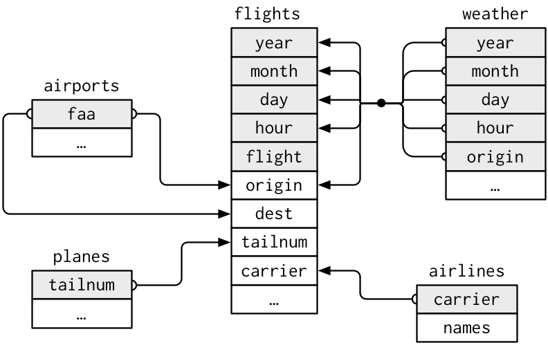
R for Data Science - nycflights13 data relationships
We can now begin to solve our question in pieces:
- We need to know which planes were single engine
single_engine <- planes %>% filter(engines == 1)
- We need to identify which column can be used to link our single engine data with our flights data.
# identify column names in common between single_engine and flights
names(single_engine)[names(single_engine) %in% names(flights)]
#> [1] "tailnum" "year"
Tailnum is going to identify our planes between our two datasets. It
is possible to use multiple keys in joins - however in our case
flights$year refers to the year of the flight, but
single_engine$year refers to the year of the aircraft.
- We now need to join with our flights data so that only the flights involving planes with single engines remain.
single_engine_flights <- inner_join(flights, single_engine, by = "tailnum")

names(single_engine_flights)
#>  [1] "year.x"         "month"          "day"            "dep_time"
#>  [5] "sched_dep_time" "dep_delay"      "arr_time"       "sched_arr_time"
#>  [9] "arr_delay"      "carrier"        "flight"         "tailnum"
#> [13] "origin"         "dest"           "air_time"       "distance"
#> [17] "hour"           "minute"         "time_hour"      "year.y"
#> [21] "type"           "manufacturer"   "model"          "engines"
#> [25] "seats"          "speed"          "engine"
Notice that we have year.x and year.y columns, this is because there
were columns that had the same name in our datasets, but were not
representing the same data. We can make these more informative going
forward by redoing our join and this time supplying a
suffix parameter so we know which dataset the columns
originally were from
single_engine_flights <- inner_join(flights, single_engine, by = "tailnum", suffix = c("_flight", "_plane"))

names(single_engine_flights)
#>  [1] "year_flight"    "month"          "day"            "dep_time"
#>  [5] "sched_dep_time" "dep_delay"      "arr_time"       "sched_arr_time"
#>  [9] "arr_delay"      "carrier"        "flight"         "tailnum"
#> [13] "origin"         "dest"           "air_time"       "distance"
#> [17] "hour"           "minute"         "time_hour"      "year_plane"
#> [21] "type"           "manufacturer"   "model"          "engines"
#> [25] "seats"          "speed"          "engine"
- Now we’ll find the total distance for each carrier
total_single_engine_carrier_distance <- single_engine_flights %>%
  group_by(carrier) %>%
summarise(total_distance = sum(distance))- And now we need to add on the carrier names and sort the result so the longest distance is first. This time we’ll do it using pipe.
total_single_engine_carrier_distance %>%
  inner_join(airlines, by = 'carrier') %>%
  arrange(desc(total_distance))
#> # A tibble: 4 × 3
#>   carrier total_distance name
#>   <chr>            <dbl> <chr>
#> 1 B6             1077735 JetBlue Airways
#> 2 AA              882584 American Airlines Inc.
#> 3 MQ              244203 Envoy Air
#> 4 FL                2286 AirTran Airways Corporation
From this we can see that JetBlue Airways flew the longest distance using single-engine planes.